Variational mechanics in one and two dimensions

We develop heuristic derivations of two alternative principles of least action. A particle moving in one dimension can reverse direction at will if energy conservation is the only criterion. Such arbitrary changes in the direction of motion are eliminated by demanding that the Maupertuis–Euler abbreviated action, equal to the area under the momentum versus position curve in phase space, has the smallest possible value consistent with conservation of energy. Minimizing the abbreviated action predicts particle trajectories in two and three dimensions and leads to the more powerful Hamilton principle of least action, which not only generates conservation of energy, but also predicts motion even when the potential energy changes with time. Introducing action early in the physics program requires modernizing the current obscure and confusing terminology of variational mechanics. © 2005 American Association of Physics Teachers.

Contents

• I. PREVIEW: LIST OF ACTORS IN ORDER OF APPEARANCE
• II. ABBREVIATED ACTION IN ONE DIMENSION
• III. ABBREVIATED ACTION IN TWO DIMENSIONS
• IV. CONSTRUCTING THE TRAJECTORY
• V. JUST PLAIN ACTION
• VI. CONSTRUCTING THE WORLDLINE
• VII. TIME-DEPENDENT POTENTIAL ENERGY
• VIII. SELF-DESCRIPTIVE TERMINOLOGY
• ACKNOWLEDGMENTS
• REFERENCES
• FIGURES
• FOOTNOTES

An asteroid named Woolsthorpe, roaming between the orbits of Mars and Jupiter, appears to be heading in the general direction of Earth. Should we worry? Given the initial position and velocity of the asteroid and data on the shifting positions of nearby asteroids and distant planets as well as the Sun, Isaac Newton (1642–1727) tells us how the asteroid's velocity changes from instant to instant. By summing the resulting increments, we derive the reassuring prediction that Woolsthorpe will pass farther from Earth than our Moon. Newton answers the questions, "What happens next?"

Newton's incremental construction of the path is not so useful in basketball. Given the initial position and speed (and therefore energy) of the ball, the shooter wants to know what direction of launch will place the center of the basketball at the center of the basketball hoop. Both launch and target points are defined in space. Pierre-Louis Moreau de Maupertuis (1698–1759) and Leonard Euler (1707–1783) offer us their abbreviated principle of least action¹ to find the direction in which to launch the basketball.² Maupertuis and Euler answer the question, "Starting from here, how do we get to there?"

None of the three, Newton, Maupertuis, or Euler, could easily manage a Moon shot. The spaceship launches from its Earth orbit and coasts toward an orbit around the Moon. The Earth and Moon are in motion; the spaceship must arrive at the correct point in space when the Moon is nearby. Both launch and arrival specify events, indexed by time as well as by location. William Rowan Hamilton (1805–1865) provides the principle of least action, which can be used to find the required initial speed (and therefore energy) and direction of launch to reach the Moon orbit safely. Hamilton answers the question, "Starting from here now, how do we get to there then?"

As these three examples demonstrate, least action principles and Newton's laws form a powerful combination for the analysis of motion. Introductory mechanics courses currently employ Newton's vector laws of motion to engage questions similar to that posed by the hurtling asteroid. Least action principles, which are powerful tools in analyzing tasks similar to basketball and Moon shots, are introduced only in advanced mechanics courses which use difficult and abstract mathematics.

Earlier we have advocated starting the study of mechanics with conservation of energy, leading more or less directly to the principle of least action.³ We have since come to believe that momentum and Newton's laws deserve their present prominence in introductory physics, but that action principles can and should be introduced early, not only because they prepare the way for advanced mechanics courses, but also because they are fundamental tools in many fields of physics such as optics, electromagnetism, quantum mechanics, and relativity.

We do not yet have a strategy for introducing least action; this paper presents a first step toward that goal, a story line that such an introduction might follow. Our purpose is to stimulate discussion about introducing action principles early in the physics curriculum.

A stone moves with varying velocity in the y direction in a time-independent potential such as that due to gravity near the Earth's surface. Conservation of energy is (almost) sufficient to predict its motion in one dimension. The total energy E is

where the kinetic energy is represented by K, the symbol used in most introductory physics texts, U(y) is the potential energy, and v is the speed of the stone. This speed is approximated by vs/t, where s is the incremental distance covered by the stone in time t. For motion in the y-direction s=|y|. Manipulation of Eq. (1) leads to a relation between s and the corresponding time increment t:

For the uniform gravitational field near the Earth's surface, the differential version of Eq. (2) easily integrates to an analytic solution. But analytic solutions are available for only a limited number of potential energy functions. In contrast, the one-dimensional motion in all reasonable potentials is easily predicted using a simple numerical integration method based on Eq. (2) or improved numerical methods, which are straightforward, conceptually transparent, and already in the toolkits of many undergraduates.

Interactive displays can encourage students to manipulate fundamental concepts in mechanics, as illustrated in Fig. 1:⁴ (bottom panel) the energy diagram; (central panel) the position versus time curve called the worldline, a term which should be introduced long before relativity; (top panel) the velocity versus position diagram, which becomes the phase diagram when the velocity is multiplied by the mass.

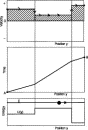Figure 1.

The particle motion shown in Fig. 1 leads to a worldline AB that exhibits two "kinks," sharp changes in slope. The energy diagram shows that each kink occurs at the location of an abrupt change in the potential energy. The result is a sudden change in the velocity (the velocity is the inverse slope of the worldline), displayed in the velocity versus position graph. So the kinks in the worldline AB have a physical basis as idealizations.

In two and three dimensions, conservation of energy alone is not sufficient to determine the particle motion. The reason is that energy is a scalar which tells us only the magnitude s of the next step along the trajectory, not its direction. Predicting motion in two and three dimensions also requires the direction of the next step. Equation (2) gives a preview of this difficulty for one-dimensional motion. Conservation of energy yields s, the magnitude of the incremental displacement y. For one-dimensional motion the two possible directions are either –v for which y=–s or +v with y=+s. For both cases Eq. (2) gives only the magnitude s. These two possibilities are illustrated in Fig. 2. Both worldlines AB and AC satisfy conservation of energy. Worldline AB is the sensible one, the worldline that meets our expectations as shown in Fig. 1. In contrast, along the worldline AC the particle reverses direction twice in the vicinity of the position y_o, keeping the same speed and therefore the same kinetic energy. In principle, a particle moving in one dimension can reverse direction at will if energy conservation were the only criterion.

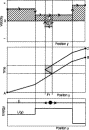Figure 2.

The worldline AC is unacceptable, but not because it has kinks in it; the worldline AB also has kinks, sudden changes in velocity at the positions of idealized jumps in the potential energy as shown in the bottom panel. Rather, the worldline AC is unacceptable because it contains spontaneous reversals of the direction unrelated to changes in the potential energy. Worse is that there is no logical or physical safeguard against an arbitrary number of such spontaneous reversals of direction. It is clear that our understanding of particle motion in terms of conservation of energy alone is incomplete.

What other principles can be used to reject spontaneous reversals of direction? Conservation of momentum applies to an isolated system; the presence of a potential energy function due to an external source tells us that the system is not isolated. Newton's second law allows us to reject spontaneous reversals of direction. In Fig. 2 the reversal occurs where the potential energy is uniform, so the application of Newton's second law says that v(F/m)t=[(–dU/dy)/m]t=0 and prohibits these reversals. However, we seek an alternative procedure for predicting motion which employs conservation of scalar energy instead of Newton's vector law.

In Fig. 2, worldlines AB and AC have identical slopes (corresponding to identical velocities) everywhere except in the dot-shaded region of the spacetime diagram. So the velocity versus position curves provide a useful tool for highlighting the difference between these two possible motions. Pay attention to the area under the velocity versus position graphs in Figs. 1 and 2. The worldline AB generates the diagonally shaded area in Fig. 2, identical to the diagonally shaded area in Fig. 1. The velocities along the worldline AC are identical to those along AB except at the double jog near y_o. The resulting multiple-valued velocity versus position graph for AC encloses the same diagonally shaded area, and in addition encloses the dot-shaded areas labeled 1 and 2. (Area 1 is enclosed twice during the motion described by worldline AC.)

The area enclosed by the velocity versus position graph provides a handle by which to understand the difference between the realistic motion described by worldline AB and the unrealistic motion depicted by worldline AC. One way to eliminate spontaneous reversals of motion as a possible feature of the worldline is to demand that the area under the v versus y curve have the smallest possible value consistent with conservation of energy.

The momentum versus position diagram is called the phase diagram, and the trajectory in this diagram is called the phase curve. The area under the phase curve is the abbreviated action⁵ and is given the symbol S_o:

The reason for "abbreviated" will become apparent. The condition that eliminates the velocity-reversing jogs in the worldline now becomes: The particle moves so that the abbreviated action has the smallest possible value, subject to conservation of energy.

The area under the phase curve can be expressed as:⁶

Equation (4) uses the speed v and the distance ds instead of the velocity dy/dt and the displacement dy, because all incremental contributions to the integral are positive. For a particle moving in the positive y-direction in Fig. 2, its velocity has the same positive value as the speed v and the incremental displacement dy is positive and equals ds. Therefore the incremental contribution to the area is positive: mv ds. For a particle moving in the negative y-direction, its velocity (–v) is the negative of the speed v and the incremental displacement (dy=–ds) is the negative of the incremental distance ds. As a result, the incremental contribution to the area also is positive: m(–v)(–ds)=mvds.

The abbreviated principle of least action requires that the value of S_o be a minimum for the actual motion of a particle. In other words, from all possible nearby trajectories in space beginning at a fixed launch point and ending at a fixed target point, the particle traverses the trajectory with the smallest value of S_o. The construction of the phase curve, m times the velocity plotted in Fig. 2, requires conservation of energy, so conservation of energy is assumed in the abbreviated principle of least action. Note that the abbreviated principle of least action is a prescription for the trajectory as a whole, which is different in character from the prescription provided by Newton's second law.

The action integral, Eq. (4), also applies in two and three dimensions, where v is the speed and ds is the incremental distance along the two- or three-dimensional trajectory. The minimization of the action S_o selects from possible nearby energy-conserving trajectories the actual trajectory followed by the particle. For simplicity, we assume that the potential energy function varies with the y-coordinate only, for example, U(y)=mgy for a basketball.

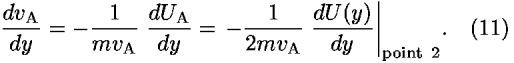
To find a trajectory y(x) that leads to a minimum value of S_o in Eq. (4) for fixed initial and final locations, we divide and conquer. If the entire action integral is a minimum, then the contribution to the integral from each infinitesimal portion of the trajectory also must be a minimum.⁷ Figure 3 shows the initial infinitesimal portion of a trajectory in the xy plane (the trajectory is not a worldline). The dotted curve represents the beginning portion of a trial trajectory approximated by line segments A, B, and C. This approximation can be made as accurate as desired by choosing points 1–4 sufficiently close together.

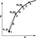Figure 3.

Figure 4 shows an alternative initial portion of the trial trajectory derived by displacing point 2 in the y-direction. Conservation of energy and the local value of the potential energy fix the average speed of the particle along each segment in Figs. 3 and 4. Finding the portion of the trajectory given by segments A and B reduces to using algebra and elementary calculus to find the y-position of the center point 2 that minimizes the abbreviated action for these segments. Equation (4) expresses the abbreviated action S_oAB along segments A and B:

The lower case s in s_A and s_B refers to the incremental length of each segment; v_A and v_B are the corresponding average speeds whose values are derived from conservation of energy. To find the minimum value of the abbreviated action S_oAB, we take the derivative of both sides of Eq. (5) with respect to y (all remaining coordinates are fixed) and set the result equal to zero:

The notation in Fig. 4 leads to expressions for each of the terms in Eq. (6). The Pythagorean theorem tells us how the length s_A varies with y, the independent vertical coordinate of point 2:

Equation (6) requires the derivative of s_A with respect to y:

Conservation of energy determines the value of the average speed along each segment:

Here U_A is the average potential energy along segment A, approximated as the average of the values at its two ends:

The derivative of v_A with respect to y comes from Eqs. (9) and (10):

The time t₂–t₁ taken to traverse segment A equals the length of the segment s_A divided by the average speed v_A across the segment:

The expressions for segment A from Eqs. (7,8,9,10,11,12) plus the corresponding expressions for segment B allow us to recast Eq. (6) into the form

and lead to a powerful result which is hidden in the notation:

The numerator on the right side of Eq. (14) is the difference between the average y-momenta p_yA and p_yB on segments A and B. The denominator approximates the time of travel from the midpoint of segment A to the midpoint of segment B. The right side of Eq. (14) thus approximates the time derivative of the y-component of the particle momentum. The left side of Eq. (14) is the value of the quantity –dU/dy at the displaced point 2, the expression for the y-component of the force in a given potential. Thus Eq. (14) is an approximation to the y-component of Newton's second law of motion, an approximation that becomes exact for infinitesimal segments:

where the dot over the momentum p indicates the time derivative.

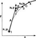Figure 4.

Alternatively, minimizing the abbreviated action S_oAB along segments A and B by varying the x-coordinate of the center point 2 leads to

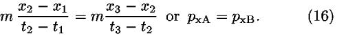
Equation (16) expresses the conservation of x-momentum between segments A and B and is in accord with Newton's second law for the case in which the potential energy U is not a function of x, namely F_x=–dU/dx=0=_x so that p_x does not change with time.

If your allegiance is to Newton's second law, then you can treat Eqs. (15) and (16) as validating the abbreviated principle of least action when the energy is conserved. Alternatively, you can view Eqs. (15) and (16) as demonstrating the priority of the abbreviated principle of least action, because Newton's second law and conservation of momentum both grow out of it. We prefer to emphasize here the consistency among these different predictors of motion.

The procedure outlined in Sec. III easily adapts to constructing the trajectory of a particle with fixed endpoints and conserved total energy. Let the segments in the left-hand graph in Fig. 5 be infinitesimal portions of a trial trajectory drawn arbitrarily to connect the fixed launch point (point 1) with the fixed target point (not shown) for a particle of fixed total energy. Points 2–4 are a sequence of adjacent points along the beginning of the trial trajectory. As explained in the caption of Fig. 5, we first vary the y-coordinate and then the x-coordinate of each intermediate point to find the location that minimizes S_o along the two adjacent segments. Repeat the sweep along the entire modified trial trajectory until no further displacements of the intermediate points occur.⁸ The resulting path approximates the trajectory taken by the particle. Equations (14,15,16) tell us that at every intermediate point along the resulting trajectory Newton's second law holds.

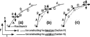Figure 5.

The total energy and the value of the potential energy at the launch point yields the launch speed and the completed trajectory determines the initial direction of motion at launch. Thus the abbreviated principle of least action tells us how to launch the particle (speed and direction) from the fixed initial point so that it will arrive at the target.

The trajectory alone does not fully describe the motion. A complete description includes not only the trajectory, but also the time at which the particle passes each point along the trajectory, plotted as the worldline. The basketball player does not care when the center of the ball reaches the center of the hoop.⁹ Nevertheless, our procedure can easily be extended to find the time at which the particle passes each point along the trajectory. Equation (12) yields the time t₂–t₁ along segment A and similar equations give the time along later segments, resulting in the total time from the launch to any point on the trajectory. The combination of the trajectory plus the time at each point on the trajectory, embodied in the worldline, provides a complete description of the flight of the basketball.

A standard result of projectile motion for a value of energy greater than the minimum is the possibility of two trajectories between the launch and target, one path higher and of longer duration, the other flatter and of shorter duration. The technique for constructing trajectories described here will discover only one of these, depending on the initial arbitrarily chosen trial path. Finding the second trajectory requires a different initial trial function. This case, with its alternative analytic solutions, is a good one for introducing students to the qualitative skills required to guess trial trajectories when multiple paths are possible.

A small additional step reveals a truly remarkable and general expression due to Hamilton,¹⁰ for which the name action stands powerfully alone, with no modifier. This action earns the symbol S, without a subscript, and is defined as:

The following simple expression relates the action S to the abbreviated action S_o:¹¹

Equation (18) can be derived from an extension of Eq. (4):

The first integral on the left in Eq. (19) is a summation along the trajectory in space, from the launch to the target. In contrast, the last integral on the right in Eq. (19) multiplies twice the kinetic energy along each segment of the path by the incremental time required to traverse that segment and sums the result. The last integral can be regarded as a summation along the worldline. Adding and subtracting the potential energy function U on the right side of Eq. (19) gives the result:

The integral containing K–U on the right-hand side of Eq. (20) is the action S, as defined in Eq. (17). In the last integral on the right-hand side of Eq. (20) the total energy E=K+U does not change with time, and therefore the integral equals (t_final–t_initial)E; Eq. (18) follows immediately.

Equation (18) deserves close scrutiny. Suppose that the procedure outlined in Sec. IV leads to the actual trajectory in space that minimizes S_o on the left-hand side of Eq. (18). Section IV tells us how to complete the worldline, which gives the time of arrival at the target, t_final. Hence minimizing S_o on the left side of Eq. (18) gives us everything about the right side, including the worldline along which the integral S is taken and the time limits of the integration.

Instead of employing the abbreviated action S_o on the left side of Eq. (18), we try using the action S on the right side to predict the motion. The action integral S is taken along the worldline between the fixed initial and final events. We boldly postulate the principle of least action, which requires that the integral S in Eq. (17) have a minimum value for the worldline taken by the particle between fixed events, that is, with known elapsed time t_final–t_initial on the right side of Eq. (18). The new least action principle implies a change from the original constraints—fixed endpoints in space and fixed energy—to physically less restrictive constraints—fixed initial and final events in spacetime. For all nearby worldlines anchored on the same initial and final events, we predict that the particle moves along that worldline for which the value of S is a minimum.

Specifying the arrival event means specifying in advance the arrival time t_final. But this final time affects the kinetic energy K along different parts of the worldline required to meet the specified deadline and therefore affects the value of the total energy E. It turns out that minimizing the value of the action S not only validates the conservation of energy along the actual worldline, but also yields the value of the conserved energy E.

To simplify our study of the action integral S, we return to one-dimensional motion and seek a worldline y(t) that minimizes the value of S between fixed initial and final events. The trial worldline, a portion of which is shown in Fig. 6, need not have a direction-reversing jog in it, as was required for alternative worldlines when the value of the energy was fixed in advance (see Fig. 2). Our expectation that the derived energy-conserving worldline be smooth for a smooth potential energy function will turn out to be justified.

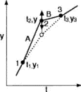Figure 6.

Figure 6 approximates a portion of the trial worldline with incremental straight segments, with the independent coordinate t along the horizontal axis, just as Fig. 4 plots the independent coordinate x along the horizontal axis. Figure 6 focuses on two adjacent segments, A and B, that lie somewhere along this trial worldline. We temporarily fix events 1 and 3 while moving event 2 in the y-direction to study the effect of this displacement on the value of the action S_AB summed along segments A and B. A student exercise shows that the outcome is the same: the y-component of Newton's law F_y=_y, Eq. (15). Therefore minimizing the action S is equivalent to invoking Newton's second law.

In finding the worldline using the principle of least action, we did not assume in advance that energy is conserved for a potential energy U(y). Nevertheless, if the expression U for potential energy does not contain the time explicitly, the principle of least action includes the conservation of energy. The actual worldline of least action must satisfy a minimal condition not only with respect to the space coordinates, but also with respect to time. The equation expressing a zero derivative of S with respect to time is nothing but conservation of energy. This result follows from varying the t-location of event 2 in Fig. 6 while keeping its y-coordinate constant. The approximate expression for the action S_AB along worldline segments A and B is

where t is the time of event 2. The minimum value of Eq. (21) follows from setting its derivative with respect to t equal to zero. The average kinetic energy along segment A is

The time derivative of (t₃–t)K_B in Eq. (21) yields the result K_B.

Because the potential energy is a function of space coordinate y only, the average potential energy U_A along segment A does not change its value with the time displacement of event 2. Therefore the time derivative of the term in Eq. (21) that includes U_A becomes

The time derivative of (t₃–t)U_B in Eq. (21) yields the result –U_B.

If we substitute Eqs. (22) and (23) for segment A plus the corresponding expressions for segment B into the expression for the derivative of Eq. (21) with respect to the time t of event 2 and set the result equal to zero, we obtain

Equation (24) can be written as

which says that energy is conserved along segments A and B.

The worldline of a particle derives from the principle of least action using an iterative process similar to that used to find the trajectory in Sec. IV and illustrated in Fig. 5. The sequence of steps is essentially identical to that used for the abbreviated action when the original x, y coordinates for a trajectory become the t, y coordinates for a worldline, as shown by the alternative t, y coordinate axes in Fig. 5. We first move the y-coordinate and then the t-coordinate of each intermediate event to minimize the action along the adjacent pair of segments, sweeping repeatedly along the worldline between fixed initial and final events until the intermediate events no longer move on the spacetime diagram. The resulting segmented worldline approximates the worldline followed by the particle.

The limit-taking process of applying the principle of least action to each pair of adjacent segments in sequence, when multiple sweeps along the worldline are completed, satisfies Newton's second law and matches the value of the energy between every adjacent pair of segments, Eq. (25), and therefore determines the value of the energy on every segment of the worldline. The value of E derived from the principle of least action multiplied by the total elapsed time (fixed at the beginning of the analysis) completes the right side of Eq. (18). Knowledge of the worldline yields the trajectory, which allows us to evaluate the integral S_o on the left side of Eq. (18) for the now-determined value of the energy E. In brief, either side of Eq. (18) predicts the motion of a particle in a time-independent potential U: Minimizing S_o on the left side for a fixed energy determines the trajectory; minimizing S on the right side for a fixed time lapse determines the worldline.

One payoff of describing motion using a scalar energy and a scalar action is the straightforward generalization of the analysis to motion in three dimensions, in which the potential energy function has the general form U(x,y,z). This generalization requires only a simple extension of the analysis in Secs. III–VI. The partial derivative with respect to any spatial coordinate that minimizes the action or the abbreviated action leads to the corresponding component of Newton's second law; the partial derivative with respect to time that minimizes action leads to the conservation of energy.

In many cases the potential energy changes with time. For example, the gravitational potential at a point in space between the Earth and Moon changes as the Moon moves. This time-varying potential can change the energy E of a spaceship moving through that point. Newton's second law relates the acceleration to the instantaneous force described by the spatial derivative of the potential energy, Eq. (14). Therefore Newton's law applies from instant to instant, even if the potential changes with time.

Constructing the worldline using the principle of least action involves a variation of the y-coordinate of each intermediate event on the worldline, while holding constant the time of that event, as illustrated in Fig. 6. Our approximation takes the value of the potential energy along each segment to be the average of its two endpoints. The endpoints in Fig. 6 are events, and the approximation corresponding to Eq. (10) is

The variation of the y-coordinate of event 2 does not change the time t₂ of that event, so the minimum action again leads to Newton's second law. Indeed, it can be shown that the principle of least action is equivalent to Newton's second law for nondissipative systems.¹² Therefore the principle of least action is also valid for time-varying potentials. In contrast, the principle of abbreviated action assumes conservation of energy, so it cannot predict motion when the potential energy varies with time.

Does the principle of least action also lead to a correct accounting of the changing particle energy when the potential energy changes with time? The analysis is a simple extension of the one that leads to Eq. (25). Minimizing the action along segments A and B in Fig. 6 requires varying the t-coordinate of point 2, while keeping its y-coordinate constant. Equations (21) and (22) remain valid for the time-dependent potential energy, but Eq. (23) is altered using Eq. (26). Setting the time derivative of the action equal to zero leads to

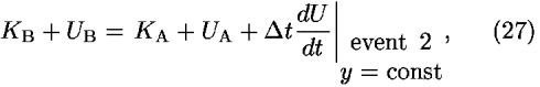
where t is the elapsed time as the particle moves between the midpoints of the adjacent segments. Equation (27) correctly approximates the increase in the total energy of the particle as it passes across segments A and B.

Another important type of motion takes place under a constraint, for example, a bead sliding without friction along a rod that rotates at a constant rate.¹³ In such motion the forces of constraint typically change the energy of the particle. Newton's laws are awkward for describing motion under such a constraint because of its vector nature (and for additional reasons). In contrast, the scalar principle of least action treats such constrained motion with simplicity and power.

Before we can move the two principles of least action to a position earlier in the physics curriculum, we need to update the language of variational mechanics, making its terminology self-consistent, transparent, and easy to understand. The present terminology of variational mechanics is clogged with the accumulated sludge of ancient trial and error and the detritus of genius. Our Murky Terminology Award goes to adjectives describing constraints of motion: holonomic, semiholonomic, rheonomous, and scleronomous. Terms encrusted with the barnacles of eminent contributors' names obstruct the flow of understanding. Who could know from the names Hamilton's principal function or Lagrange's equations what each is about, how they are used, or why they might be important?¹⁴ Students should not be forced to master a polyglot language before they can revel in the simplicity and power of action.

The terms for our mechanics tools should be self-descriptive. The self-descriptive name of an object, principle, or application recalls for us and drives home its key feature every time we read, speak, hear, or apply it. First prize for a self-descriptive name goes to black hole, which summarizes the properties of a mighty astronomical object. The term black hole is not only descriptive but also exciting, firing the public imagination. The original study of collapsed gravitational structures did not lead to this term. The name was long sought, stumbled upon, recognized, and promoted by John Archibald Wheeler.¹⁵

Why not replace abbreviated action with the term fixed-energy action or trajectory action? Could Lagrange's equations become local equations of motion? It may be difficult to find self-descriptive names for fundamental concepts of a field, but these names should at least be snappy and motivating. We would not be writing a paper promoting the use of Hamilton's principal function, but Landau and Lifschitz, and later Feynman, renamed it action, cutting the number of syllables by three-quarters and invigorating the field.¹⁶

Even the field of mechanics needs new names. Classical mechanics currently means nonquantum mechanics; special and general relativity are classical subjects. This paper focuses on the more restricted field of Newtonian mechanics, which predicts nonrelativistic, nonquantum motion. Newton's greatness is not enhanced by using his name to smother magisterial contributions by Euler, Lagrange, Jacobi, Hamilton, and others.

The authors wish to thank Kenneth Ford, Don S. Lemons, and Jon Ogborn for useful discussions and helpful suggestions.

1. We use the name least action instead of the technically correct stationary action for several reasons: (a) Many cases involve a local minimum of the action. (b) The value of the action is always a minimum for a sufficiently small segment of the curve. (c) The word least is self-descriptive, but stationary requires additional explanation. (d) The word least does not lead to the error that the value of either form of action, Eqs. (4) and (17), can be a maximum for an actual path, which it cannot. (e) Least action is the name most often used in the historical literature on the subject. We recommend that the term stationary action be introduced, with careful explanation, not long after the term least action itself. first citation in article
   
2. For linear gravitational potential energy near the Earth's surface, we can integrate Newton's second law to derive an analytic expression for the basketball trajectory and hence the required direction of launch. However, in more complicated potentials we are reduced to trial and error to find a path that passes through the basket. Minimizing the Maupertuis–Euler abbreviated action finds the trajectory in one stroke. A similar comment applies to the Moon shot described in the following paragraph: Minimizing Hamilton's action gives us the worldline directly. first citation in article
   
3. Jozef Hanc and Edwin F. Taylor, "From conservation of energy to the principle of least action: A story line," Am. J. Phys. 72, 514–521 (2004). [ISI] first citation in article
   
4. Derivations of the action outlined in this paper were stimulated by an interactive Java program developed by one of the authors (ST). This display numerically integrates Eq. (2), solving for the one-dimensional motion of a particle in a time-independent potential. In its extended form, the program shows all three panels in Fig. 1. The program is available at http://vscience.euweb.cz/worldlines/Worldlines.html. first citation in article
   
5. The name abbreviated action and the symbol S_o are used by L. D. Landau and E. M. Lifschitz, Mechanics (Butterworth-Heinemann, London, 1999), Vol. 1, 3rd ed., p. 141, and Herbert Goldstein, Charles Poole, and John Safko, Classical Mechanics (Addison–Wesley, San Francisco, 2002), 3rd ed., pp. 359, 434. We have named the corresponding variational principle the abbreviated principle of least action, rather than the more technically correct principle of least abbreviated action, believing that "least abbreviated" might be incorrectly interpreted as "augmented." first citation in article
   
6. Wolfgang Yourgrau and Stanley Mandelstam, Variational Principles in Dynamics and Quantum Theory (Dover, New York, 1979), pp. 24–29. first citation in article
   
7. Richard P. Feynman, Robert B. Leighton, and Matthew Sands, The Feynman Lectures on Physics (Addison–Wesley, San Francisco, 1964), Vol. II, p. 19-8. first citation in article
   
8. The minimization procedure for constructing a trajectory or worldline described in the caption to Fig. 5 is conceptually simple but not the most effective in practice. In both cases it is more efficient to start with a trial segmented curve with equal increments along the horizontal axis. Then we vary only the y-coordinates of intermediate points to minimize the action, obtaining the actual path. The minimization of action with respect to coordinates along the horizontal axis is not necessary because the result is just points uniformly distributed on the horizontal axis, which was our initial assumption. We do not discuss here the proof of this statement or the convergence of the algorithm, because it goes beyond the scope of the present paper. first citation in article
   
9. According to the official rules of the National Basketball Association, a basket is scored after the final buzzer provided the ball is launched before the buzzer sounds. first citation in article
   
10. For Hamilton's development of the principle of least action, see two of his papers at http://www.maths.tcd.ie/pub/HistMath/People/Hamilton/Dynamics/. first citation in article
    
11. Landau and Lifschitz, Ref. 5, p. 141, Eq. (44.3); Goldstein et al., Ref. 5, p. 359. first citation in article
    
12. Our derivation can be reversed to show the equivalence of Newton's second law and the principle of least action. See also Goldstein et al., Ref. 5, p. 35. first citation in article
    
13. The example of a bead sliding along a uniformly rotating rod is in Goldstein et al., Ref. 5, pp. 28–29. Additional example is a pendulum whose string support is slowly pulled up through a small hole. See Cornelius Lanczos, The Variational Principle of Mechanics (Dover, New York, 1986), 4th ed., p. 124. first citation in article
    
14. Further examples of name-encrusted terminology: d'Alembert's principle, Hamiltonian, Hamilton's principle, Hamilton's equations, Hamilton–Jacobi equation, Jacobi identity, Jacobi principle, Jacobi condition, Jacobi's theorem, Lagrangian, Poisson bracket, Poisson's equations, Hilbert integral, Legendre condition, Poincare invariants, Cartheodory's method, Bernoulli's method, Clebsch condition, Clebsch relation, Clebsch transformation, Descartes–Snell rule, Noether's theorem, Rayleigh's dissipation function, Routh's procedure, Staeckel conditions, Weierstrass condition, Weierstrass–Erdmann corner condition. first citation in article
    
15. Kip S. Thorne, Black Holes and Time Warps: Einstein's Outrageous Legacy (Norton, New York, 1994), pp. 256–257; John Archibald Wheeler with Kenneth Ford, Geons, Black Holes, and Quantum Foam: A Life in Physics (Norton, New York, 1998), pp. 296–297. first citation in article
    
16. Landau and Lifschitz, Ref. 5, Chap. 1; Landau and Lifschitz rechristened Hamilton's principal function as the action in the first Russian edition in 1958, and in a 1940 textbook, a precursor of Ref. 5; See also Feynman, Ref. 7. first citation in article
    

Full figure

Fig. 1. Screen shot of the interactive program showing the energy and potential energy diagram in the bottom panel, the worldline (the plot relating position and time) in the middle panel, and a plot of velocity versus position y in the top panel. The diagonal shading of the area under the velocity versus position graph has been added for use in comparing alternative motions depicted in Fig. 2. First citation in article

Full figure

Fig. 2. Two sequential spontaneous reversals of direction with the same speed near position y_o satisfy conservation of energy but are unphysical. The original worldline AB shown in Fig. 1 generates the diagonally shaded area under the velocity curve at the top of Fig. 1. The worldline AC not only generates the same enclosed area, but also adds the superposed dot-shaded areas labeled 1 and 2. Area 1 is enclosed twice in this process. First citation in article

Full figure

Fig. 3. The infinitesimal initial portion of the curved trajectory of a particle in the xy plane (dotted line) might represent the first millisecond of motion of a particle that starts at fixed point 1. The dotted trajectory is approximated by three connected straight segments A, B, C. First citation in article

Full figure

Fig. 4. We vary the y-position of point 2 to minimize the abbreviated action along segments A and B. First citation in article

Full figure

Fig. 5. Construction of the trajectory y(x) in two dimensions. The initial segments are shown. Point 1 is the fixed launch point. (a) We first vary the y-coordinate and then the x-coordinate of point 2 to find the location that minimizes the value of the abbreviated action S_oAB along segments A and B. (b) We move point 2 to that new location, then vary the y coordinate, then the x-coordinate of point 3 to find the location that minimizes the value of S_oBC along segments B and C. (c and continuation) We move point 3 to that new location and continue moving later points on the trial trajectory all the way to the fixed final point (the target, not shown). We repeatedly sweep the entire trial trajectory until the intermediate points no longer change. The resulting trajectory approximates that taken by the particle. As described in Sec. VII, a similar construction with y and t coordinates approximates the worldline which minimizes Hamilton's action S. First citation in article

Full figure

Fig. 6. Two adjacent infinitesimal segments A and B are chosen arbitrarily along the trial worldline of a particle moving in one dimension in a time-independent potential. Events 1 and 3 are temporarily fixed, while the y-coordinate of event 2 is displaced in order to find its position 2 for the minimum value of the action along segments A and B. First citation in article

^aElectronic mail: jozef.hanc@tuke.sk

^bAuthor to whom correspondence should be addressed. Electronic mail: eftaylor@mit.edu

^cElectronic mail: tuleja@stonline.sk

Up: Issue Table of Contents
Go to: Previous Article | Next Article
Other formats: HTML (smaller files) | PDF (107 kB)

REFERENCES

Citation links [e.g., Phys. Rev. D 40, 2172 (1989)] go to online journal abstracts. Other links (see Reference Information) are available with your current login. Navigation of links may be more efficient using a second browser window.