American Journal of Physics, Vol. 72, No. 4, pp. 514–521, April 2004
©2004 American Association of Physics Teachers. All rights reserved.
From conservation of energy to the principle of least action: A story line
Jozef Hanca)
Technical University, Faculty of Metallurgy, Department of Metal Forming, Vysokoskolska 4, 042 00 Kosice, Slovakia
Edwin F. Taylorb)
Massachusetts Institute of Technology, Department of Physics, Cambridge, Massachusetts 02139
Received: 27 August 2003; accepted: 5 December 2003We outline a story line that introduces Newtonian mechanics by employing conservation of energy to predict the motion of a particle in a one-dimensional potential. We show that incorporating constraints and constants of the motion into the energy expression allows us to analyze more complicated systems. A heuristic transition embeds kinetic and potential energy into the still more powerful principle of least action. © 2004 American Association of Physics Teachers.
Contents
I. INTRODUCTION
An eight sentence history of Newtonian mechanics1 shows how much the subject has developed since Newton introduced F = dp/dt in the second half of the 1600s.2 In the mid-1700s Euler devised and applied a version of the principle of least action using mostly geometrical methods. In 1755 the 19-year-old Joseph-Louis Lagrange sent Euler a letter that streamlined Euler's methods into algebraic form. "[A]fter seeing Lagrange's work Euler dropped his own method, espoused that of Lagrange, and renamed the subject the calculus of variations."3 Lagrange, in his 1788 Analytical Mechanics,4 introduced what we call the Lagrangian function and Lagrange's equations of motion. About half a century later (1834–1835) Hamilton published Hamilton's principle,5 to which Landau and Lifshitz6 and Feynman7 reassigned the name principle of least action.8 Between 1840 and 1860 conservation of energy was established in all its generality.9 In 1918 Noether10 proved several relations between symmetries and conserved quantities. In the 1940s Feynman11 devised a formulation of quantum mechanics that not only explicitly underpins the principle of least action, but also shows the limits of validity of Newtonian mechanics.
Except for conservation of energy, students in introductory physics are typically introduced to the mechanics of the late 1600s. To modernize this treatment, we have suggested12 that the principle of least action and Lagrange's equations become the basis of introductory Newtonian mechanics. Recent articles discuss how to use elementary calculus to derive Newton's laws of motion,13 Lagrange's equations,14 and examples of Noether's theorem15 from the principle of least action, describe the modern rebirth of Euler's methods16 and suggest ways in which upper undergraduate physics classes can be transformed using the principle of least action.17
How are these concepts and methods to be introduced to undergraduate physics students? In this paper we suggest a reversal of the historical order: Begin with conservation of energy and graduate to the principle of least action and Lagrange's equations. The mathematical prerequisites for the proposed course include elementary trigonometry, polar coordinates, introductory differential calculus, partial derivatives, and the idea of the integral as a sum of increments.
The story line presented in this article omits most details and is offered for discussion, correction, and elaboration. We do not believe that a clear story line guarantees student understanding. On the contrary, we anticipate that trials of this approach will open up new fields of physics education research.
II. ONE-DIMENSIONAL MOTION: ANALYTIC SOLUTIONS
We start by using conservation of energy to analyze particle motion in a one-dimensional potential. Much of the power of the principle of least action and its logical offspring, Lagrange's equations, results from the fact that they are based on energy, a scalar. When we start with conservation of energy, we not only preview more advanced concepts and procedures, but also invoke some of their power. For example, expressions for the energy which are consistent with any constraints automatically eliminate the corresponding constraint forces from the equations of motion. By using the constraints and constants of the motion, we often can reduce the description of multi-dimensional systems to one coordinate, whose motion can then be found using conservation of energy. Equilibrium and statics also derive from conservation of energy.
We first consider one-dimensional motion in a uniform vertical gravitational field. Heuristic arguments lead to the expression mgy for the potential energy. We observe, with Galileo, that the velocity of a particle in free fall from rest starting at position y = 0 decreases linearly with time:  = –gt, where we have expressed the time derivative by a dot over the variable. This relation integrates to the form
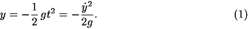
We multiply Eq. (1) by mg and rearrange terms to obtain the first example of conservation of energy:

where the symbol E represents the total energy and the symbols K and U represent the kinetic and potential energy, respectively.
A complete description of the motion of a particle in a general conservative one-dimensional potential follows from the conservation of energy. Unfortunately, an explicit function of the position versus time can be derived for only a fraction of such systems. Students should be encouraged to guess analytic solutions, a powerful general strategy because any proposed solution is easily checked by substitution into the energy equation. Heuristic guesses are assisted by the fact that the first time derivative of the position, not the second, appears in the energy conservation equation.
The following example illustrates the guessing strategy for linear motion in a parabolic potential. This example also introduces the potential energy diagram, a central feature of our story line and an important tool in almost every undergraduate subject.
A. Harmonic oscillator
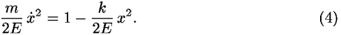
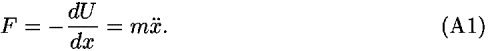
Our analysis begins with a qualitative prediction of the motion of a particle in a parabolic potential (or in any potential with motion bounded near a single potential energy minimum). If we consider the potential energy diagram for a fixed total energy, we can predict that the motion will be periodic. For a parabolic potential (Fig. 1) conservation of energy is expressed as

We rearrange Eq. (3) to read
Equation (4) reminds us of the trigonometric identity,

We set  =
=  t and equate the right-hand sides of Eqs. (4) and (5) and obtain the solution
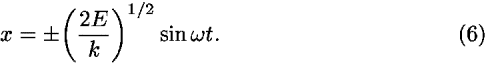
If we take the time derivative of x in Eq. (6) and use it to equate the left-hand sides of Eqs. (4) and (5), we find that18
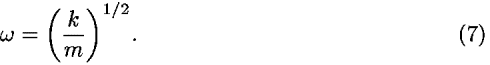
The fact that does not depend on the total energy E of the particle means that the period is independent of E and hence independent of the amplitude of oscillation described by Eq. (6). The simple harmonic oscillator is widely applied because many potential energy curves can be approximated as parabolas near their minima.
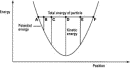 Figure 1.
 At this point, it would be desirable to introduce the concept of the worldline, a position versus time plot that completely describes the motion of a particle.
III. ACCELERATION AND FORCE
In the absence of dissipation, the force can be defined in terms of the energy. We start with conservation of energy:

We take the time derivative of both sides and use the chain rule:
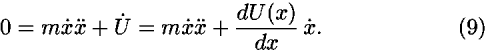
By invoking the tendency of a ball to roll downhill, we can define force as the negative spatial derivative of the potential,
![<i>m</i><i>x</i>-double_dot [equivalent] <i>F</i> = –((<i>d</i><i>U</i>(<i>x</i>))/<i>d</i><i>x</i>),](energy_to_action_files/514_1m10.gif)
from which we see that F = –kx for the harmonic potential and F = –mg for the gravitational force near the earth's surface.
IV. NONINTEGRABLE MOTIONS IN ONE DIMENSION
We guessed a solution for simple harmonic motion, but it is important for students to know that for most mechanical systems, analytical solutions do not exist, even when the potential can be expressed analytically. For these cases, our strategy begins by asking students to make a detailed qualitative prediction of the motion using the potential energy diagram, for example, describing the velocity, acceleration, and force at different particle positions, such as A through F in Fig. 1.
The next step might be to ask the student to plot by hand a few sequential points along the worldline using a difference equation derived from energy conservation corresponding to Eq. (3),
![<i>d</i><i>x</i> = {(2/<i>m</i>) [<i>E</i> – <i>U</i>(<i>x</i>)]}<sup>1/2</sup><i>d</i><i>t</i>,](energy_to_action_files/514_1m11.gif)
where U(x) describes an arbitrary potential energy. The process of plotting necessarily invokes the need to specify the initial conditions, raises the question of accuracy as a function of step size, and forces an examination of the behavior of the solution at the turning points. Drawing the resulting worldline can be automated using a spreadsheet with graphing capabilities, perhaps comparing the resulting approximate curve with the analytic solution for the simple harmonic oscillator.
After the drudgery of these preliminaries, students will welcome a more polished interactive display that numerically integrates the particle motion in a given potential. On the potential energy diagram (see Fig. 2), the student sets up initial conditions by dragging the horizontal energy line up or down and the particle position left or right. The computer then moves the particle back and forth along the E-line at a rate proportional to that at which the particle will move, while simultaneously drawing the worldline (upper plot of Fig. 2).
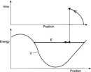 Figure 2.
 V. REDUCTION TO ONE COORDINATE
The analysis of one-dimensional motion using conservation of energy is powerful but limited. In some important cases we can use constraints and constants of the motion to reduce the description to one coordinate. In these cases we apply our standard procedure: qualitative analysis using the (effective) potential energy diagram followed by interactive computer solutions. We illustrate this procedure by some examples.
A. Projectile motion
For projectile motion in a vertical plane subject to a uniform vertical gravitational field in the y-direction, the total energy is

The potential energy is not a function of x; therefore, as shown in the following, momentum in the x-direction, px, is a constant of the motion. The energy equation becomes
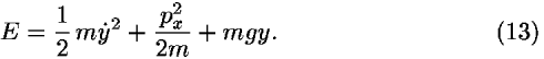
In Newtonian mechanics the zero of the energy is arbitrary, so we can reduce the energy to a single dimension y by making the substitution:
![<i>E</i><sup>[prime]</sup> = <i>E</i>–(<i>p</i><sub><i>x</i></sub><sup>2</sup>/2<i>m</i>) = (1/2) <i>m</i><i>y</i>-dot<sup>2</sup> + <i>m</i><i>g</i><i>y</i>.](energy_to_action_files/514_1m14.gif)
Our analysis of projectile motion already has applied a limited version of a powerful theorem due to Noether.19 The version of Noether's theorem used here says that when the total energy E is not an explicit function of an independent coordinate, x for example, then the function ![[partial-derivative]](energy_to_action_files/part.gif) E/
E/ is a constant of the motion.20 We have developed a simple, intuitive derivation of this version of Noether's theorem. The derivation is not included in this brief story line.
The above strategy uses a conservation law to reduce the number of dimensions. The following example uses constraints to the same end.
B. Object rolling without slipping
Two-dimensional circular motion and the resulting kinetic energy are conveniently described using polar coordinates. The fact that the kinetic energy is an additive scalar leads quickly to its expression in terms of the moment of inertia of a rotating rigid body. When the rotating body is symmetric about an axis of rotation and moves perpendicularly to this axis, the total kinetic energy is equal to the sum of the energy of rotation plus the energy of translation of the center of mass. (This conclusion rests on the addition of vector components, but does not require the parallel axis theorem.) Rolling without slipping is a more realistic idealization than sliding without friction.
We use these results to reduce to one dimension the description of a marble rolling along a curved ramp that lies in the x-y plane in a uniform gravitational field. Let the marble have mass m, radius r, and moment of inertia Imarble. The nonslip constraint tells us that v = r. Conservation of energy leads to the expression:

where
The motion is described by the single coordinate y. Constraints are used twice in this example: explicitly in rolling without slipping and implicitly in the relation between the height y and the displacement along the curve.
C. Motion in a central gravitational field
We analyze satellite motion in a central inverse-square gravitational field by choosing the polar coordinates r and  in the plane of the orbit. The expression for the total energy is

The angle does not appear in Eq. (17). Therefore we expect that a constant of the motion is given by E/ , which represents the angular momentum J. (We reserve the standard symbol L for the Lagrangian, introduced later in this paper.)
![(([partial-derivative]<i>E</i>)/([partial-derivative] <i>phi</i>-dot)) = <i>m</i><i>r</i><sup>2</sup><i>phi</i>-dot = <i>J</i>.](energy_to_action_files/514_1m20.gif)
We substitute the resulting expression for into Eq. (17) and obtain

Students employ the plot of the effective potential energy Ueff(r) to do the usual qualitative analysis of radial motion followed by computer integration. We emphasize the distinctions between bound and unbound orbits. With additional use of Eq. (18), the computer can be programmed to plot a trajectory in the plane for each of these cases.
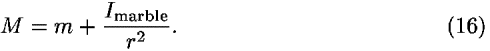
D. Marble, ramp, and turntable
This system is more complicated, but is easily analyzed by our energy-based method and more difficult to treat using F = ma. A relatively massive marble of mass m and moment of inertia Imarble rolls without slipping along a slot on an inclined ramp fixed rigidly to a light turntable which rotates freely so that its angular velocity is not necessarily constant (see Fig. 3). The moment of inertia of the combined turntable and ramp is Irot. We assume that the marble stays on the ramp and find its position as a function of time.
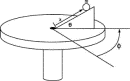 Figure 3.
 We start with a qualitative analysis. Suppose that initially the turntable rotates and the marble starts at rest with respect to the ramp. If the marble then begins to roll up the ramp, the potential energy of the system increases, as does the kinetic energy of the marble due to its rotation around the center of the turntable. To conserve energy, the rotation of the turntable must decrease. If instead the marble begins to roll down the ramp, the potential energy decreases, the kinetic energy of the marble due to its rotation around the turntable axis decreases, and the rotation rate of the turntable will increase to compensate. For a given initial rotation rate of the turntable, there may be an equilibrium value at which the marble will remain at rest. If the marble starts out displaced from this value, it will oscillate back and forth along the ramp.
More quantitatively, the square of the velocity of the marble is

Conservation of energy yields the relation

where M indicates the marble's mass augmented by the energy effects of its rolling along the ramp, Eq. (16). The right side of Eq. (21) is not an explicit function of the angle of rotation . Therefore our version of Noether's theorem tells us that E/ is a constant of the motion, which we recognize as the total angular momentum J:
![(([partial-derivative]<i>E</i>)/([partial-derivative] <i>phi</i>-dot)) = (<i>I</i><sub>rot</sub> + <i>M</i><i>x</i><sup>2</sup> cos<sup>2</sup> <i>theta</i>)<i>phi</i>-dot = <i>J</i>.](energy_to_action_files/514_1m24.gif)
If we substitute into Eq. (21) the expression for from Eq. (22), we obtain

The values of E and J are determined by the initial conditions. The effective potential energy Ueff(x) may have a minimum as a function of x, which can result in oscillatory motion of the marble along the ramp. If the marble starts at rest with respect to the ramp at the position of minimum effective potential, it will not move along the ramp, but execute a circle around the center of the turntable.
VI. EQUILIBRIUM AND STATICS: PRINCIPLE OF LEAST POTENTIAL ENERGY
Our truncated story line does not include frictional forces or an analysis of the tendency of systems toward increased entropy. Nevertheless, it is common experience that motion usually slows down and stops. Our use of potential energy diagrams makes straightforward the intuitive formulation of stopping as a tendency of a system to reach equilibrium at a local minimum of the potential energy. This result can be formulated as the principle of least potential energy for systems in equilibrium. Even in the absence of friction, a particle placed at rest at a point of zero slope in the potential energy curve will remain at rest. (Proof: An infinitesimal displacement results in zero change in the potential energy. Due to energy conservation, the change in the kinetic energy must also remain zero. Because the particle is initially at rest, the zero change in kinetic energy forbids displacement.) Equilibrium is a result of conservation of energy.
Here, as usual, Feynman is ahead of us. Figure 4 shows an example from his treatment of statics.21 The problem is to find the value of the hanging weight W that keeps the structure at rest, assuming a beam of negligible weight. Feynman balances the decrease in the potential energy when the weight W drops 4![[double-prime]](energy_to_action_files/Prime-script.gif) with increases in the potential energy for the corresponding 2 rise of the 60 lb weight and the 1 rise in the 100 lb weight. He requires that the net potential energy change of the system be zero, which yields
with increases in the potential energy for the corresponding 2 rise of the 60 lb weight and the 1 rise in the 100 lb weight. He requires that the net potential energy change of the system be zero, which yields
![–4<sup>[double-prime]</sup>W + 2<sup>[double-prime]</sup>(60 lb) + 1<sup>[double-prime]</sup>(100 lb) = 0,](energy_to_action_files/514_1m26.gif)
or W = 55 lb. Feynman calls this method the principle of virtual work, which in this case is equivalent to the principle of least potential energy, both of which express conservation of energy.
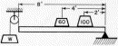 Figure 4.
 There are many examples of the principle of minimum potential energy, including a mass hanging on a spring, a lever, hydrostatic balance, a uniform chain suspended at both ends, a vertically hanging slinky,22 and a ball perched on top of a large sphere.
VII. FREE PARTICLE. PRINCIPLE OF LEAST AVERAGE KINETIC ENERGY
For all its power, conservation of energy can predict the motion of only a fraction of mechanical systems. In this and Sec. VIII we seek a principle that is more fundamental than conservation of energy. One test of such a principle is that it leads to conservation of energy. Our investigations will employ trial worldlines that are not necessarily consistent with conservation of energy.
We first think of a free particle initially at rest in a region of zero potential energy. Conservation of energy tells us that this particle will remain at rest with zero average kinetic energy. Any departure from rest, say by moving back and forth, will increase the average of its kinetic energy from the zero value. The actual motion of this free particle gives the least average kinetic energy. The result illustrates what we will call the principle of least average kinetic energy.
Now we view the same particle from a reference frame moving in the negative x-direction with uniform speed. In this frame the particle moves along a straight worldline. Does this worldline also satisfy the principle of least average kinetic energy? Of course, but we can check this expectation and introduce a powerful graphical method established by Euler.16
We fix two events A and C at the ends of the worldline (see Fig. 5) and vary the time of the central event B so that the kinetic energy is not the same on the legs labeled 1 and 2. Then the time average of the kinetic energy K along the two segments 1 and 2 of the worldline is given by
![<i>K</i><sub>avg</sub> = ((<i>K</i><sub>1</sub><i>t</i><sub>1</sub> + <i>K</i><sub>2</sub><i>t</i><sub>2</sub>)/<i>t</i><sub>total</sub>) = (1/<i>t</i><sub>total</sub>) [(1/2) <i>m</i><i>v</i><sub>1</sub><sup>2</sup><i>t</i><sub>1</sub>+(1/2) <i>m</i><i>v</i><sub>2</sub><sup>2</sup><i>t</i><sub>2</sub>].](energy_to_action_files/514_1m27.gif)
We multiply both sides of Eq. (25) by the fixed total time and recast the velocity expressions using the notation in Fig. 5:

We find the minimum value of the average kinetic energy by taking the derivative with respect to the time t of the central event:

From Eq. (27) we obtain the equality

As expected, when the time-averaged kinetic energy has a minimum value, the kinetic energy for a free particle is the same on both segments; the worldline is straight between the fixed initial and final events A and C and satisfies the principle of minimum average kinetic energy. The same result follows if the potential energy is uniform in the region under consideration, because the uniform potential energy cannot affect the kinetic energy as the location of point B changes on the spacetime diagram.
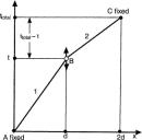 Figure 5.
 In summary, we have illustrated the fact that for the special case of a particle moving in a region of zero (or uniform) potential energy, the kinetic energy is conserved if we require that the time average of the kinetic energy has a minimum value. The general expression for this average is
![<i>K</i><sub>avg</sub> = (1/<i>t</i><sub>total</sub>) [integral]<sub>(entire; path; )</sub> <i>K</i> <i>d</i><i>t</i>.](energy_to_action_files/514_1m31.gif)
In an introductory text we might introduce at this point a sidebar on Fermat's principle of least time for the propagation of light rays.
Now we are ready to develop a similar but more general law that predicts every central feature of mechanics.
VIII. PRINCIPLE OF LEAST ACTION
Section VI discussed the principle of least potential energy and Sec. VII examined the principle of least average kinetic energy. Along the way we mentioned Fermat's principle of least time for ray optics. We now move on to the principle of least action, which combines and generalizes the principles of least potential energy and least average kinetic energy.
A. Qualitative demonstration
We might guess (incorrectly) that the time average of the total energy, the sum of the kinetic and potential energy, has a minimum value between fixed initial and final events. To examine the consequences of this guess, let us think of a ball thrown in a uniform gravitational field, with the two events, pitch and catch, fixed in location and time (see Fig. 6). How will the ball move between these two fixed events? We start by asking why the baseball does not simply move at constant speed along the straight horizontal trajectory B in Fig. 6. Moving from pitch to catch with constant kinetic energy and constant potential energy certainly satisfies conservation of energy. But the straight horizontal trajectory is excluded because of the importance of the averaged potential energy.
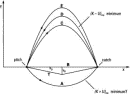 Figure 6.
 We need to know how the average kinetic energy and average potential energy vary with the trajectory. We begin with the idealized triangular path T shown in Fig. 6. If we assume a fixed time between pitch and catch and that the speed does not vary wildly along the path, the kinetic energy of the particle is approximately proportional to the square of the distance covered, that is, proportional to the quantity x + y using the notation in Fig. 6. The increase in the kinetic energy over that of the straight path is proportional to the square of the deviation y0, whether that deviation is below or above the horizontal path. But any incremental deviation from the straight-line path can be approximated by a superposition of such triangular increments along the path. As a result, small deviations from the horizontal path result in an increase in the average kinetic energy approximately proportional to the average of the square of the vertical deviation y0.
The average potential energy increases or decreases for trajectories above or below the horizontal, respectively. The magnitude of the change in this average is approximately proportional to the average deviation y0, whether this deviation is small or large.
We can apply these conclusions to the average of E = K + U as the path departs from the horizontal. For paths above the horizontal, such as C, D, and E in Fig. 6, the averages of both K and U increase with deviation from the horizontal; these increases have no limit for higher and higher paths. Therefore, no upward trajectory minimizes the average of K + U. In contrast, for paths that deviate downward slightly from the horizontal, the average K initially increases slower than the average U decrease, leading to a reduction in their sum. For paths that dip further, however, the increase in the average kinetic energy (related to the square of the path length) overwhelms the decrease in the average potential energy (which decreases only as y0). So there is a minimum of the average of K + U for some path below the horizontal. The path below the horizontal that satisfies this minimum is clearly not the trajectory observed for a pitched ball.
Suppose instead we ask how the average of the difference K–U behaves for paths that deviate from the horizontal. By an argument similar to that in the preceding paragraph, we see that no path below the horizontal can have a minimum average of the difference. But there exists a path, such as D, above the horizontal for which the average of K–U is a minimum. For the special case of vertical launch, students can explore this conclusion interactively using tutorial software.23
B. Analytic demonstration
We can check the preceding result analytically in the simplest case we can imagine (see Fig. 7). In a uniform vertical gravitational field a marble of mass m rolls from one horizontal surface to another via a smooth ramp so narrow that we may neglect its width. In this system the potential energy changes just once, halfway between the initial and final positions.
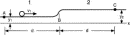 Figure 7.
 The worldline of the particle will be bent, corresponding to the reduced speed after the marble mounts the ramp, as shown in Fig. 8. We require that the total travel time from position A to position C have a fixed value ttotal and check whether minimizing the time average of the difference K–U leads to conservation of energy:
![(<i>K</i> – <i>U</i>)<sub>avg</sub> = (1/<i>t</i><sub>total</sub>) [(<i>K</i> – <i>U</i>)<sub>1</sub><i>t</i><sub>1</sub> + (<i>K</i> – <i>U</i>)<sub>2</sub><i>t</i><sub>2</sub>].](energy_to_action_files/514_1m33.gif)
We define a new symbol S, called the action:
![<i>S</i> [equivalent] (<i>K</i> – <i>U</i>)<sub>avg</sub><i>t</i><sub>total</sub> = (<i>K</i> – <i>U</i>)<sub>1</sub><i>t</i><sub>1</sub> + (<i>K</i> – <i>U</i>)<sub>2</sub><i>t</i><sub>2</sub>.](energy_to_action_files/514_1m34.gif)
We can use the notation in Fig. 8 to write Eq. (31) in the form

where M is given by Eq. (16). We require that the value of the action be a minimum with respect to the choice of the intermediate time t:
This result can be written as
A simple rearrangement shows that Eq. (34) represents conservation of energy. We see that energy conservation has been derived from the more fundamental principle of least action. Equally important, the analysis has completely determined the worldline of the marble.
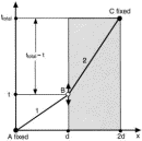 Figure 8.
 The action Eq. (31) can be generalized for a potential energy curve consisting of multiple steps connected by smooth, narrow transitions, such as the one shown in Fig. 9:

The argument leading to conservation of energy, Eq. (34), applies to every adjacent pair of steps in the potential energy diagram. The computer can hunt for and find the minimum value of S directly by varying the values of the intermediate times, as shown schematically in Fig. 10.
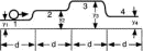 Figure 9.
 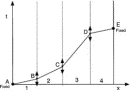 Figure 10.
 A continuous potential energy curve can be regarded as the limiting case of that shown in Fig. 9 as the number of steps increases without limit while the time along each step becomes an increment  t. For the resulting potential energy curve the general expression for the action S is
![<i>S</i> [equivalent] [integral]<sub>(entire; path; )</sub><i>L</i> <i>d</i><i>t</i> = [integral]<sub>(entire; path; )</sub>(<i>K</i> – <i>U</i>) <i>d</i><i>t</i>.](energy_to_action_files/514_1m39.gif)
Here L (= K–U for the cases we treat) is called the Lagrangian. The principle of least action says that the value of the action S is a minimum for the actual motion of the particle, a condition that leads not only to conservation of energy, but also to a unique specification of the entire worldline.
More general forms of the principle of least action predict the motion of a particle in more than one spatial dimension as well as the time development of systems containing many particles. The principle of least action can even predict the motion of some systems in which energy is not conserved.24 The Lagrangian L can be generalized so that the principle of least action can describe relativistic motion7 and can be used to derive Maxwell's equations, Schroedinger's wave equation, the diffusion equation, geodesic worldlines in general relativity, and steady electric currents in circuits, among many other applications.
We have not provided a proof of the principle of least action in Newtonian mechanics. A fundamental proof rests on nonrelativistic quantum mechanics, for instance that outlined by Tyc25 which uses the deBroglie relation to show that the phase change of a quantum wave along any worldline is equal to S/![[h-bar]](energy_to_action_files/planck.gif) , where S is the classical action along that worldline. Starting with this result, Feynman and Hibbs have shown26 that the sum-over-all-paths description of quantum motion reduces seamlessly to the classical principle of least action as the masses of particles increase.
, where S is the classical action along that worldline. Starting with this result, Feynman and Hibbs have shown26 that the sum-over-all-paths description of quantum motion reduces seamlessly to the classical principle of least action as the masses of particles increase.
Once students have mastered the principle of least action, it is easy to motivate the introduction of nonrelativistic quantum mechanics. Quantum mechanics simply assumes that the electron explores all the possible worldlines considered in finding the Newtonian worldline of least action.
IX. LAGRANGE'S EQUATIONS
Lagrange's equations are conventionally derived from the principle of least action using the calculus of variations.27 The derivation analyzes the worldline as a whole. However, the expression for the action is a scalar; if the value of the sum is minimum along the entire worldline, then the contribution along each incremental segment of the worldline also must be a minimum. This simplifying insight, due originally to Euler, allows the derivation of Lagrange's equations using elementary calculus.14 The appendix shows an alternative derivation of Lagrange's equation directly from Newton's equations.
ACKNOWLEDGMENTS
The authors acknowledge useful comments by Don S. Lemons, Jon Ogborn, and an anonymous reviewer.
APPENDIX: DERIVATION OF LAGRANGE'S EQUATIONS FROM NEWTON'S SECOND LAW
Both Newton's second law and Lagrange's equations can be derived from the more fundamental principle of least action.13,14 Here we move from one derived formulation to the other, showing that Lagrange's equation leads to F = ma (and vice versa) for particle motion in one dimension.28
If we use the definition of force in Eq. (10), we can write Newton's second law as:
We assume that m is constant and rearrange and recast Eq. (A1) to read
![((<i>d</i>(–<i>U</i>))/<i>d</i><i>x</i>)–(<i>d</i>/<i>d</i><i>t</i>) (<i>m</i><i>x</i>-dot) = ((<i>d</i>(–<i>U</i>))/<i>d</i><i>x</i>)–(<i>d</i>/<i>d</i><i>t</i>) [(<i>d</i>/(<i>d</i><i>x</i>-dot)) (((<i>m</i><i>x</i>-dot<sup>2</sup>)/2))] = 0.](energy_to_action_files/514_1m41.gif)
On the right-hand side Eq. (A2) we add terms whose partial derivatives are equal to zero:
![(([partial-derivative])/([partial-derivative]<i>x</i>)) [((<i>m</i><i>x</i>-dot<sup>2</sup>)/2) – <i>U</i>(<i>x</i>)]–(<i>d</i>/<i>d</i><i>t</i>) [(([partial-derivative])/([partial-derivative]<i>x</i>-dot)) (((<i>m</i><i>x</i>-dot<sup>2</sup>)/2) – <i>U</i>(<i>x</i>))] = 0.](energy_to_action_files/514_1m42.gif)
We then set L = K–U, which leads to the Lagrange equation in one dimension:
![(([partial-derivative]<i>L</i>)/([partial-derivative]<i>x</i>))–(<i>d</i>/<i>d</i><i>t</i>) [(([partial-derivative]<i>L</i>)/([partial-derivative]<i>x</i>-dot))] = 0.](energy_to_action_files/514_1m43.gif)
This sequence of steps can be reversed to show that Lagrange's equation leads to Newton's second law of motion for conservative potentials.
REFERENCES
Citation links [e.g., Phys. Rev. D 40, 2172 (1989)] go to online journal abstracts. Other links (see Reference Information) are available with your current login. Navigation of links may be more efficient using a second browser window.
-
We use the phrase Newtonian mechanics to mean nonrelativistic, nonquantum mechanics. The alternative phrase classical mechanics also applies to relativity, both special and general, and is thus inappropriate in the context of this paper.
first citation in article
-
Sir Isaac Newton's Mathematical Principles of Natural Philosophy and His System of the World, translated by Andrew Motte and Florian Cajori (University of California, Berkeley, 1946), p. 13.
first citation in article
-
Herman H. Goldstine, A History of the Calculus of Variations From the 17th Through the 19th Century (Springer-Verlag, New York, 1980), p. 110.
first citation in article
-
J. L. Lagrange, Analytic Mechanics, translated by Victor N. Vagliente and Auguste Boissonnade (Kluwer Academic, Dordrecht, 2001).
first citation in article
-
William Rowan Hamilton, "On a general method in dynamics, by which the
study of the motions of all free systems of attracting or repelling
points is reduced to the search and differentiation of one central
Relation or characteristic Function," Philos. Trans. R. Soci. Part II,
247–308 (1834);
"Second essay on a general method in dynamics," Part I, 95–144 (1835). Both papers are available at  http://www.emis.de/classics/Hamilton/
 .
first citation in article
.
first citation in article
-
L. D. Landau and E. M. Lifshitz, Mechanics, Course of Theoretical Physics
(Butterworth-Heinemann, London, 1976), 3rd ed., Vol. 1, Chap. 1. Their
renaming first occurred in the original 1957 Russian edition. first citation in article
-
Richard P. Feynman, Robert B. Leighton, and Matthew Sands, The Feynman Lectures on Physics (Addison-Wesley, Reading MA, 1964), Vol. II, pp. 19-8.
first citation in article
-
The technically correct term is principle of stationary action. See I. M. Gelfand and S. V. Fomin, Calculus of Variations, translated by Richard A. Silverman (Dover, New York, 2000), Chap. 7, Sec. 36.2. However, we prefer the conventional term principle of least action for reasons not central to the argument of the present paper.
first citation in article
-
Thomas H. Kuhn, "Energy conservation as an example of simultaneous discovery," in The Conservation of Energy and the Principle of Least Action, edited by I. Bernard Cohen (Arno, New York, 1981).
first citation in article
-
E. Noether, "Invariante Variationprobleme," Nach. v.d. Ges. d. Wiss zu Goettingen, Mathphys. Klasse, 235–257 (1918);
English translation by M. A. Tavel, "Invariant variation problem," Transp. Theory Stat. Phys. 1 (3), 183–207 (1971). [ISI]
first citation in article
-
Richard P. Feynman, "Space-time approach to non-relativistic quantum mechanics," Rev. Mod. Phys. 20 (2), 367–387 (1948).
first citation in article
-
Edwin F. Taylor, "A call to action," Am. J. Phys. 71 (5), 423–425 (2003). [ISI]
first citation in article
-
Jozef Hanc, Slavomir Tuleja, and Martina Hancova, "Simple derivation of
Newtonian mechanics from the principle of least action," Am. J. Phys. 71 (4), 386–391 (2003). [ISI]
first citation in article
-
Jozef Hanc, Edwin F. Taylor, and Slavomir Tuleja, "Deriving Lagrange's
equations using elementary calculus," accepted for publication in Am.
J. Phys. Preprint available at http://www.eftaylor.com.
first citation in article
-
Jozef Hanc, Slavomir Tuleja, and Martina Hancova, "Symmetries and
conservations laws: Consequences of Noether's theorem," accepted for
publication in Am. J. Phys. Preprint available at http://www.eftaylor.com.
first citation in article
-
Jozef Hanc, "The original Euler's calculus-of-variations method: Key to
Lagrangian mechanics for beginners," submitted to Am. J. Phys. Preprint
available at http://www.eftaylor.com.
first citation in article
-
Thomas A. Moore, "Getting the most action out of least action," submitted to Am. J. Phys. Preprint available at http://www.eftaylor.com.
first citation in article
-
Student exercise: Show that B cos t and C cos t + D sin t are also solutions. Use the occasion to discuss the importance of relative phase.
first citation in article
-
Benjamin Crowell bases an entire introductory treatment on Noether's theorem: Discover Physics (Light and Matter, Fullerton, CA, 1998–2002). Available at http://www.lightandmatter.com.
first citation in article
-
Noether's theorem10 implies that when the Lagrangian of a system (L = K–U for our simple cases) is not a function of an independent coordinate, x for example, then the function L/
 is a constant of the motion. This statement also can be expressed in
terms of Hamiltonian dynamics. See, for example, Cornelius Lanczos, The Variational Principles of Mechanics
(Dover, New York, 1970), 4th ed., Chap. VI, Sec. 9, statement above Eq.
(69.1). In all the mechanical systems that we consider here, the total
energy is conserved and thus automatically does not contain time
explicitly. Also the expression for the kinetic energy K is quadratic in the velocities, and the potential energy U
is independent of velocities. These conditions are sufficient for the
Hamiltonian of the system to be the total energy. Then our limited
version of Noether's theorem is identical to the statement in Lanczos. first citation in article
is a constant of the motion. This statement also can be expressed in
terms of Hamiltonian dynamics. See, for example, Cornelius Lanczos, The Variational Principles of Mechanics
(Dover, New York, 1970), 4th ed., Chap. VI, Sec. 9, statement above Eq.
(69.1). In all the mechanical systems that we consider here, the total
energy is conserved and thus automatically does not contain time
explicitly. Also the expression for the kinetic energy K is quadratic in the velocities, and the potential energy U
is independent of velocities. These conditions are sufficient for the
Hamiltonian of the system to be the total energy. Then our limited
version of Noether's theorem is identical to the statement in Lanczos. first citation in article
-
Reference 7, Vol. 1, p. 4-5.
first citation in article
-
Don S. Lemons, Perfect Form (Princeton U.P., Princeton, 1997), Chap. 4.
first citation in article
-
Slavomir Tuleja and Edwin F. Taylor, Principle of Least Action Interactive, available at http://www.eftaylor.com.
first citation in article
-
Herbert Goldstein, Charles Poole, and John Safko, Classical Mechanics (Addison-Wesley, San Francisco, 2002), 3rd ed., Sec. 2.7.
first citation in article
-
Tomas Tyc, "The de Broglie hypothesis leading to path integrals," Eur. J. Phys. 17 (5), 156–157 (1996). [Inspec]
An extended version of this derivation is available at http://www.eftaylor.com.
first citation in article
-
R. P. Feynman and A. R. Hibbs, Quantum Mechanics and Path Integrals (McGraw–Hill, New York, 1965), p. 29.
first citation in article
-
Reference 6, Chap. 1; Ref. 24, Sec. 2.3; D. Gerald Jay Sussman and Jack Wisdom, Structure and Interpretation of Classical Mechanics (MIT, Cambridge, 2001), Chap. 1.
first citation in article
-
Ya. B. Zeldovich and A. D. Myskis, Elements of Applied Mathematics, translated by George Yankovsky (MIR, Moscow, 1976), pp. 499–500.
first citation in article
CITING ARTICLES
This list contains links to other online articles that cite the article currently being viewed.
-
Hamilton's principle: Why is the integrated difference of the kinetic and potential energy minimized?
Alberto G. Rojo, Am. J. Phys. 73, 831 (2005)
-
Variational mechanics in one and two dimensions
Jozef Hanc et al., Am. J. Phys. 73, 603 (2005)
FIGURES
Full figure (6 kB)Fig. 1. The potential energy diagram is central to our treatment and requires a difficult conceptual progression from a ball rolling down a hill pictured in an x-y diagram to a graphical point moving along a horizontal line of constant energy in an energy-position diagram. Making this progression allows the student to describe qualitatively, but in detail, the motion of a particle in a one-dimensional potential at arbitrary positions such as A through F. First citation in article
Full figure (7 kB)Fig. 2. Mockup of an interactive computer display of the worldline derived numerically from the energy and the potential energy function. First citation in article
Full figure (8 kB)Fig. 3. System of marble, ramp, and turntable. First citation in article
Full figure (6 kB)Fig. 4. Feynman's example of the principle of virtual work. First citation in article
Full figure (10 kB)Fig. 5. The time of the middle event is varied to determine the path of the minimum time-averaged kinetic energy. First citation in article
Full figure (10 kB)Fig. 6. Alternative trial trajectories of a pitched ball. For path D the average of the difference K–U is a minimum. First citation in article
Full figure (4 kB)Fig. 7. Motion across a potential energy step. First citation in article
Full figure (8 kB)Fig. 8. Broken worldline of a marble rolling across steps connected by a narrow ramp. The region on the right is shaded to represent the higher potential energy of the marble on the second step. First citation in article
Full figure (5 kB)Fig. 9. A more complicated potential energy diagram, leading in the limit to a potential energy curve that varies smoothly with position. First citation in article
Full figure (6 kB)Fig. 10. The computer program temporarily fixes the end events of a two-segment section, say events B and D, then varies the time coordinate of the middle event C to find the minimum value of the total S, then varies D while C is kept fixed, and so on. (The end-events A and E remain fixed.) The computer cycles through this process repeatedly until the value of S does not change further because this value has reached a minimum for the worldline as a whole. The resulting worldline approximates the one taken by the particle. First citation in article
FOOTNOTES
aElectronic mail: jozef.hanc@tuke.sk
bAuthor to whom correspondence should be addressed. Electronic mail: eftaylor@mit.edu
Up: Issue Table of Contents
Go to: Previous Article | Next Article
Other formats: HTML (smaller files) | PDF (200 kB)
 Full figure (6 kB)
 Full figure (7 kB)
 Full figure (8 kB)
 Full figure (6 kB)
 Full figure (10 kB)
 Full figure (10 kB)
 Full figure (4 kB)
 Full figure (8 kB)
 Full figure (5 kB)
 Full figure (6 kB)
![[ISI]](http://link.aip.org/link/?&l_creator=fthtml&l_dir=FWD&l_rel=CITES&from_key=AJPIAS000072000004000514000001&from_keyType=CVIPS&from_loc=AIP&to_j=TTSPB4&to_v=1&to_p=183&to_loc=ISI&to_url=http%3A%2F%2Fgateway.isiknowledge.com%2Fgateway%2FGateway.cgi%3FGWVersion%3D2%26SrcAuth%3DAIP%26SrcApp%3DAIP%26DestLinkType%3DFullRecord%26KeyUT%3DA1971L153400002%26DestApp%3DWOS_CPL%26SrcURL%3Dhttp%253A%252F%252Flink.aip.org%252Flink%252F%253FAJP%252F72%252F514%252F1%26SrcImageURL%3Dhttp%253A%252F%252Fimages.isiknowledge.com%252FWoK3%252FImages%252FLinks%252FAIP_Ret.gif)
![[ISI]](http://link.aip.org/link/?&l_creator=fthtml&l_dir=FWD&l_rel=CITES&from_key=AJPIAS000072000004000514000001&from_keyType=CVIPS&from_loc=AIP&to_j=AJPIAS&to_v=71&to_p=423&to_loc=ISI&to_url=http%3A%2F%2Fgateway.isiknowledge.com%2Fgateway%2FGateway.cgi%3FGWVersion%3D2%26SrcAuth%3DAIP%26SrcApp%3DAIP%26DestLinkType%3DFullRecord%26KeyUT%3D000182386500001%26DestApp%3DWOS_CPL%26SrcURL%3Dhttp%253A%252F%252Flink.aip.org%252Flink%252F%253FAJP%252F72%252F514%252F1%26SrcImageURL%3Dhttp%253A%252F%252Fimages.isiknowledge.com%252FWoK3%252FImages%252FLinks%252FAIP_Ret.gif)
![[ISI]](http://link.aip.org/link/?&l_creator=fthtml&l_dir=FWD&l_rel=CITES&from_key=AJPIAS000072000004000514000001&from_keyType=CVIPS&from_loc=AIP&to_j=AJPIAS&to_v=71&to_p=386&to_loc=ISI&to_url=http%3A%2F%2Fgateway.isiknowledge.com%2Fgateway%2FGateway.cgi%3FGWVersion%3D2%26SrcAuth%3DAIP%26SrcApp%3DAIP%26DestLinkType%3DFullRecord%26KeyUT%3D000181806900015%26DestApp%3DWOS_CPL%26SrcURL%3Dhttp%253A%252F%252Flink.aip.org%252Flink%252F%253FAJP%252F72%252F514%252F1%26SrcImageURL%3Dhttp%253A%252F%252Fimages.isiknowledge.com%252FWoK3%252FImages%252FLinks%252FAIP_Ret.gif)